We’ve spent a great deal of time in past articles discussing the merits of portfolio optimization. In this article we will examine the merits and challenges of portfolio optimization in the context of one of the most challenging investment universes: Managed Futures.
Futures exhibit several features that make them challenging from a portfolio optimization perspective. In particular, there can be mathematical issues with large correlation matrices, and certain futures markets may exhibit high correlation in certain periods. However, for practitioners that are willing to make the effort, the extreme diversity offered by futures markets represents a lucrative opportunity to improve results through portfolio optimization.
Seeking diversity
Why are we convinced that diversity produces opportunity? We are motivated by the Fundamental Law of Active Management described by (Grinold 1989), which states that the risk-adjusted performance of a strategy is a mathematical function of skill and the square-root of breadth.

Where IR is information ratio, IC is information coefficient and breadth is the number of independent bets placed by the manager. For our purpose we can substitute Sharpe ratio for information coefficient because we are focused on absolute performance, not performance relative to a benchmark. Information coefficient quantifies skill by measuring the correlation between a strategy’s signals and subsequent results.
Breadth is a more nebulous concept. Grinold described breadth as the number of securities times the number of trades. However, (Polakow and Gebbie 2006) raise the issue that, “The square root of N in mathematical statistics implies ‘independence’ amongst statistical units (here bets) rather than simply the notion of ‘separate bets’ as is most often implied” in the finance literature.
It is therefore insufficient to simply add more securities in an effort to increase breadth and expand one’s Sharpe ratio. Rather, investors must account for the fact that correlated securities are, by definition, not independent. This prompts questions about how to quantify breadth – the number of independent sources of risk or “bets” – in the presence of correlations.
Quantifying breadth
All things equal investors seeking to improve results should seek to maximize the breadth that is available to them. We will show that traditional methods do a relatively poor job of maximizing breadth and diversification, and that a portfolio’s maximum potential can usually only be reached through optimization.
It’s illustrative to examine the number of independent bets that are expressed when portfolios are formed using traditional versus more advanced optimization methods. We will quantify the number of independent bets by taking the square of the Diversification Ratio of the portfolio.
(Choueifaty and Coignard 2008) showed that the Diversification Ratio of a portfolio is the ratio of the weighted sum of asset volatilities to the portfolio volatility after accounting for diversification.

This is intuitive because if all of the assets in the portfolio are correlated, the weighted sum of their volatilities would equal the portfolio volatility, and the Diversification Ratio would be 1. As the assets become less correlated, the portfolio volatility will decline due to diversification, while the weighted sum of constituent volatilities will remain the same, causing the ratio to rise. At the point where all assets are uncorrelated (zero pairwise correlations), every asset in the portfolio represents an independent source of risk.
(Choueifaty, Froidure, and Reynier 2012) demonstrate that the number of independent risk factors expressed in a portfolio is equal to the square of the Diversification Ratio of the portfolio. Thus, we can find the number of independent risk factors in a portfolio as a function of the weights in each asset and the asset covariances, which allow us to calculate the portfolio volatility.
There are many ways to form futures portfolios. Futures are defined by their underlying exposures, which can range from extremely low volatility instruments like Japanese government bonds (JGB) to very high volatility commodities like natural gas. With such large differences in risk between futures contracts, few managers would choose to hold contracts in equal weight.
Maximizing breadth
Traditional risk weighting
Perhaps the most common portfolio formation method among futures managers is to weight assets by the inverse of their volatility subject to a target risk. Contracts with low volatility would receive a larger capital allocation and vice versa. Exposure to each asset is calculated in the following way:
wi = σT/σi
where wi is the portfolio’s weight in market i, σT is the target volatility and σi is the estimated volatility of market i.
Consider a portfolio of JGB futures with an annualized volatility of 4% and natural gas futures with an annualized volatility of 50%. A manager targeting 10% annualized volatility from each instruments would hold 10%/4% = 250% of portfolio exposure in JGBs and 10%/50% = 20% in natural gas.
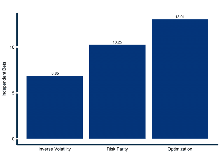
When we apply this equal volatility weighting methodology to a diversified universe of 47 futures markets across equities, fixed income, commodities and currencies we produce 6.85 independent sources of return.
Diverse correlations
The popular inverse volatility weighting method described above has the goal of dividing risk equally among diverse futures markets. Unfortunately, inverse volatility weighted portfolios are effective at diversifying risk only when all pairwise correlations between markets are equal (learn why in our seminal whitepaper, The Portfolio Optimization Machine: A General Framework for Portfolio Choice).
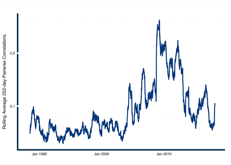
(Baltas 2015) observed that inverse volatility weighted portfolios are susceptible to major shifts in portfolio concentration as correlations change through time. This issue has become more important in the policy driven markets subsequent to the 2008 financial crisis. Figure 1 illustrates how pairwise correlations between futures markets shifted higher over the past decade.
Figure 1: Rolling average annual daily pairwise correlations across 47 futures markets.

Source: Analysis by ReSolve Asset Management. Data from CSI.
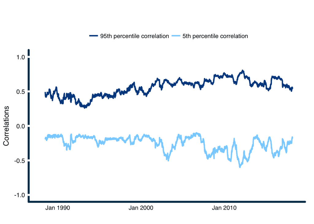
It is rarely the case that markets exhibit homogeneous correlations. Rather, segments of futures markets such as certain equity markets and some relatively fungible commodity markets like WTI and Brent crude tend to have high correlations while other markets have low or even negative correlations. Figure 2 illustrates just how diverse pairwise correlations can be across futures markets. On average the most correlated markets have had correlations of 0.56 while the least correlated markets have had correlations of -0.26.
Figure 2: Rolling 95th and 5th percentile pairwise correlations across 47 futures markets.

Source: Analysis by ReSolve Asset Management. Data from CSI.
Given that correlations exhibit such large dispersion, inverse volatility weighted portfolios will fail to produce optimally diversified portfolios. Methods for forming portfolios of futures that account for correlations require optimization1.
Toward optimal diversification
The objective of portfolio optimization is to maximize the opportunity for diversification (i.e. maximize breadth) when correlations vary over a wide range. Some assets in our futures universe have strong positive correlations while others are negatively correlated. For example, over the past year Eurostoxx and DAX have experienced a correlation of 0.93 while British Pound and Gilt futures have experienced a correlation of -0.44. All things equal, assets with low or negative correlations relative to most other assets should earn a larger weight in portfolios.
Risk parity
There are several optimization methods to choose from. (Baltas 2015) proposed using a risk parity optimization, where all assets contribute the same target risk to the portfolio after accounting for diversification. The weights for the risk parity portfolio can be found using several methods. The following method was formulated by (Spinu 2013):

The advantage of risk parity optimization is that all assets with non-zero expected returns will earn non-zero weights. Thus, the portfolio will resemble what might be produced by a traditional inverse volatility weighted approach, and will be more inuitive in constitution.
However, the risk parity portfolio will not maximize portfolio diversification, and will not explicitly maximize the expected return of the portfolio with minimal risk. A risk parity weighted portfolio of 47 futures markets would produce 10.25 independent sources of return. This is a non-trivial improvement over the traditional method’s 6.85 bets.
Mean-variance optimization
As mentioned above, (Choueifaty, Froidure, and Reynier 2012) described why the square of the portfolio’s Diversification Ratio quantifies the number of independent bets available in a portfolio. We can solve for the portfolio weights that maximize the Diversification Ratio – and thus portfolio breadth – using a form of mean-variance optimization of the following form:

where σ and Σ reference a vector of volatilities, and the covariance matrix, respectively.
The optimization maximizes the ratio of weighted-average asset volatilities to portfolio volatility after accounting for diversification. When we solve for the most diversified portfolio of futures using this method we give rise to 13.01 independent sources of return.
Figure 3: Number of independent bets from futures portfolios formed using different methods. Simulated results.

Source: Analysis by ReSolve Asset Management. Data from CSI. Simulated results.
Sharpe multiplier (M*)
Let’s take a moment to understand the importance of the results in Figure 3. Greater breadth, in the form of independent bets, is a force-multiplier on Sharpe ratios.
Recall from our discussion of the Fundamental Law of Active Management above that expected Sharpe ratio is a function of ![]() . As such portfolios formed using the risk parity method should produce Sharpe ratios
. As such portfolios formed using the risk parity method should produce Sharpe ratios ![]() times higher than the Sharpe ratio of inverse volatility weighted portfolios. And mean-variance optimized portfolios can produce Sharpe ratios
times higher than the Sharpe ratio of inverse volatility weighted portfolios. And mean-variance optimized portfolios can produce Sharpe ratios ![]() times higher. We will call this quantity the “Sharpe multiplier” M*.
times higher. We will call this quantity the “Sharpe multiplier” M*.
![Rendered by QuickLaTeX.com \[M^*=\sqrt\frac{Breadth_{Optim}}{Breadth_{Naive}}\]](https://investresolve.com/inc/ql-cache/quicklatex.com-1bf253d1ed4fce97a162c31399e6b5c7_l3.png)
To put this in perspective, if traditional diversified managed futures strategies have Sharpe ratios of 1, moving from traditional formation methods to optimization-based methods could boost Sharpe ratios to 1.38. At 10% target volatility this boosts a 10% expected annualized excess return strategy to a 13.8% expected return. Over ten years, a $1 million portfolio would be expected to grow to $2.59million using the traditional portfolio inverse volatility weighting method, but it might grow to $3.64 million if portfolios were constructed to maximize diversification. That’s an extra $1million of wealth from applying exactly the same method to select securities, but more thoughtful portfolio construction.
Breadth changes through time
Up to this point we have been calculating independent bets based on long-term average pairwise-complete correlations. Each correlation element is calculated based on the returns for each pair of futures since the inception of the shortest running futures contract.
Of course, not all futures contracts have data all the way back to 1988 and correlations are not stable through time. It is more useful to examine the true breadth – measured as number of independent bets – at each period based on point-in-time correlation estimates. Figure 4 tracks the number of independent bets produced by the three example portfolio formation methods at the end of each calendar year from 1988 through July 2018, derived from trailing 252-day (1-year) correlations.
Figure 4: Rolling number of independent bets produced by different portfolio formation methods, smoothed by trailing 252-day average. Simulated results.

Source: Analysis by ReSolve Asset Management. Data from CSI. Simulated results.
The correlation structure of our futures universe, and commensurate breadth, has fluctuated materially over the past thirty years. Breadth historically contracts when markets enter crisis periods, and expands when markets are functioning normally. In all cases however, portfolios that are optimized to maximize diversification produce considerably more breadth than traditional portfolios that ignore correlations altogether.
Notice that portfolios appear to produce greater breadth on average when they are regularly reconstituted to reflect point-in-time correlations. This is partly because the long-term average smoothes away the many different economic environments experienced by markets over the past three decades, each which produced its own diverse correlation structure. However, short-term sample correlation matrices also typically understate “true”” correlations for mathematical reasons, which are beyond the scope of this discussion. In practice, one should make adjustments to sample correlation matrices to account for sample biases2.
Across rolling annual periods, traditional inverse volatility weighted futures portfolios produced an average of 10.28 independent bets, while risk parity and optimization weighted portfolios produced an average of 16.02 and 21.91 bets respectively.

Summary and next steps
Grinold’s Fundamental Law of Active Management implies that equally skilled managers should seek to maximize breadth to boost expected performance.
Managers of futures portfolios have traditionally employed naive portfolio formation methods that ignore information about correlations. These methods, which weight markets in proportion to the inverse of volatility, are optimally diversified only if markets all have equal pairwise correlations.
Figure 2 clearly shows that correlations deviate substantially from the assumption of equality over all historical periods. As a result, traditional portfolio formation methods will render overly concentrated portfolios most of the time.
Some authors have recently proposed risk parity weighting as a solution to the problem of diverse correlations. Risk parity seeks to form portfolios such that markets contribute equal volatility after accounting for diversification. We show that risk parity produces greater breadth than traditional methods on our futures universe. However, risk parity leaves a material amount of breadth on the table.
Portfolio optimization is the only way to extract the maximum amount of breadth when markets have diverse correlations. We show that optimization produces greater breadth than both traditional methods and risk parity at every time step over the past thirty years.
The Sharpe Multiplier quantifies the expected boost to strategy performance as a result of higher breadth. Figure 5 demonstrates that optimization-based methods provide a consistent boost to expected performance. On average, optimized portfolios may exceed the performance of portfolios constructed using traditional means by up to 50%.
Our analysis prompts at least one obvious question. If optimization has such great potential to improve performance, why do most futures managers avoid it? We’ll answer it in the next article in this series. To get the most out of the articles in this series, read The Portfolio Optimization Machine: A General Framework for Portfolio Choice.
References
Baltas, Nick. 2015. “Trend-Following, Risk-Parity and the Influence of Correlations.” https://ssrn.com/abstract=2673124.
Bun, Joël, Jean-Philippe Bouchaud, and Marc Potters. 2016. “Cleaning large correlation matrices: tools from random matrix theory.” https://arxiv.org/abs/1610.08104.
Choueifaty, Yves, and Yves Coignard. 2008. “Toward Maximum Diversification.” Journal of Portfolio Management 35 (1). http://www.tobam.fr/inc/uploads/2014/12/TOBAM-JoPM-Maximum-Div-2008.pdf: 40–51.
Choueifaty, Yves, Tristan Froidure, and Julien Reynier. 2012. “Properties of the Most Diversified Portfolio.” Journal of Investment Strategies 2 (2). http://www.qminitiative.org/UserFiles/files/FroidureSSRN-id1895459.pdf: 49–70.
Grinold, Richard. 1989. “The Fundamental Law of Active Management.” 15 (3). http://jpm.iijournals.com/content/15/3/30: 30–37.
Polakow, Daniel, and Tim Gebbie. 2006. “How many independent bets are there?” https://arxiv.org/pdf/physics/0601166v1.pdf.
Spinu, Florin. 2013. “An Algorithm for Computing Risk Parity Weights.” SSRN. https://ssrn.com/abstract=2297383.
- Given that correlations exhibit such large dispersion, inverse volatility weighted portfolios will fail to produce optimally diversified portfolios. Methods for forming portfolios of futures that account for correlations require optimization^[Many futures managers use heuristic methods to help enhance diversification. For example, they may form sub-portfolios of equity markets, fixed income, currencies, and commodities. Other managers divide commodities into sub-sectors like “energies”, “grains”, “metals” or “softs”. Markets within a sector are weighted by inverse volatility, and then sector portfolios are weighted in the final portfolio by inverse volatility. This may enhance diversification properties somewhat, but pairwise correlations can vary substantially within and across sectors, suggesting this approach provides only marginal benefits relative to naive inverse volatility weighting.↩
- See (Bun, Bouchaud, and Potters 2016) for an overview of biases in sample correlation matrices.↩

